Microsoft Office Excel 2013

PivotTables and PivotCharts

99Excel Training Academy

A Microsoft Excel - Vba Training Institute, India

99Excel Training Academy

Microsoft Office Excel 2013 PivotTables & Pivot Charts

Table of Contents

Learning Objectives 4

Creating PivotTables 5

Analyzing Data with PivotTables 8

Filtering the PivotTable 9

Creating PivotCharts 11

Filtering the PivotChart 14

Using Slicers to Filter Data 16

Inserting Slicers into your PivotTable or PivotChart 16

Additional Slicer Options 18

Additional Help 19

Introduction

This booklet is the companion document to the Excel 2013: PivotTables and Pivot Charts workshop. The booklet will explain PivotTables and Pivot Charts, how to create them, and how to use them to quickly analyze large quantities of data.

Learning Objectives

After completing the instructions in this booklet, you will be able to:

Understand what PivotTables and Pivot Charts are
Insert PivotTables
Insert Pivot Charts
Filter information in your PivotTable and Pivot Chart
Understand what Slicers are
Insert Slicers
PivotTables
PivotTables are a powerful tool in Excel that will allow you to quickly summarize, sort, filter, and analyze data. They can handle large amounts of data in lists and tables by organizing data, on the fly, by different rows and columns. This is faster, and more flexible for analyzing your data, as you don’t need to rely on formulas.

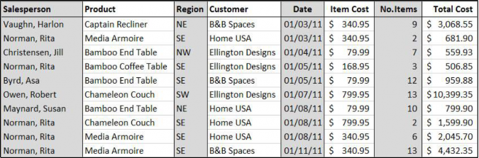
For example, you could have a spreadsheet that contains information on salespeople, products sold, regions, items sold, etc. Using a PivotTable, you can quickly organize the data so different relationships are visible (e.g. Who is the top salesperson? What product has sold the most?) (See Figure 1).

Figure 1 - Sample Sales Spreadsheet

Note: When working with PivotTables, the data should contain your titles in a single row, and the table should not contain any empty cells.

Creating PivotTables
The following will show you how to create a PivotTable using the sample sales spreadsheet as an example:
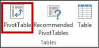
1. In the Ribbon, click on the Insert tab (See Figure 2).
  Figure 2 - Insert Tab
2. Under the Tables grouping, click on PivotTables (See Figure 3).
  
  Figure 3 - PivotTable
3. The Create PivotTable window will appear. Excel will automatically select the data it thinks you want to use to create your PivotTable (See Figure 4).
  
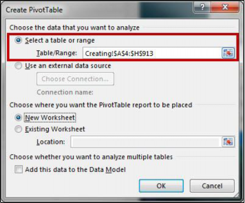
  Figure 4 - Create PivotTable Window
  
  Note: To select a different range from what Excel has suggested, click on the cell selection box () and use the mouse to select a new range.
4. Under Choose where you want the PivotTable report to be placed, select New Worksheet
  (See Figure 5).
  
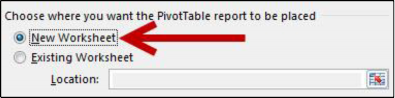
  Figure 5 - Create PivotTable on a New Worksheet
5. Click on OK.
6. The PivotTable will be created in a new worksheet (See Figure 6).
  
  Figure 6 - PivotTable Added
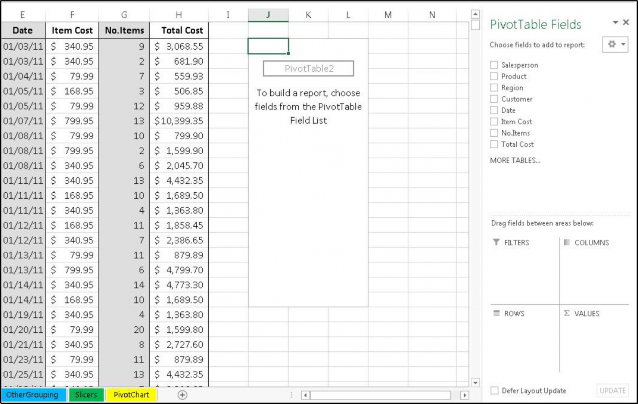
7. The PivotTable Fields will appear on the right of the screen (See Figure 7).
  
  Figure 7 - PivotTable Fields
  Analyzing Data with PivotTables
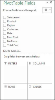
  After creating your PivotTable, the PivotTable Fields list will display the data ranges that you selected, and four areas that will make up your PivotTable (Filters, Columns, Rows, and Values). You can quickly move fields in and out of these areas to view your data in different ways.
  
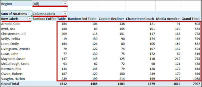
  For example, we want to use the PivotTable to analyze the data and determine how many sales a salesperson has made of each product.
  1. Drag-and-drop your fields into the filter, column, rows, and values boxes (See Figure 8).
    
    Figure 8 - Setting up Fields
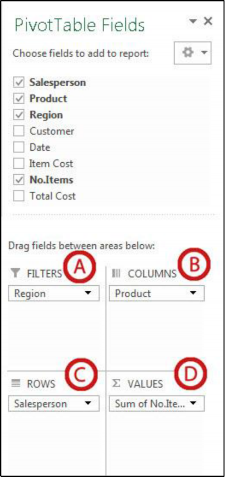
    1. Filters area fields are shown as top-level report filters above the PivotTable (See Figure 8).
    2. Columns area fields are shown as Column Labels at the top of the PivotTable (See Figure 8).
    3. Rows area fields are shown as Row Labels on the left side of the PivotTable (See Figure 8).
    4. Values area fields are shown as summarized numeric values in the PivotTable (See Figure 8).
  2. The PivotTable will change to show the fields in their respective locations, showing total sales for each sales person by product (See Figure 9).
Figure 9 - PivotTable Results

Filtering the PivotTable
The following shows how to filter information within a PivotTable:
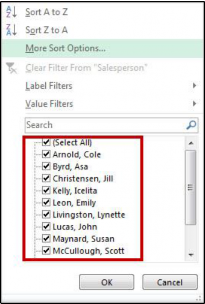
1. Next to a Field Header, click the dropdown arrow (See Figure 10).
  
  Figure 10 - Dropdown Button
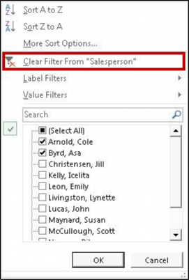
2. A Dropdown menu will appear with values for the field listed below (See Figure 11).
  
  Figure 11 – Filter Values
3. Click the checkboxes to select/deselect values that you want to filter for.
4. Click on OK to apply your filter.
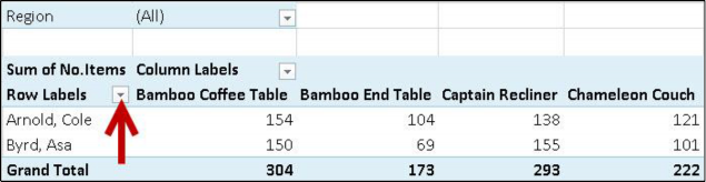
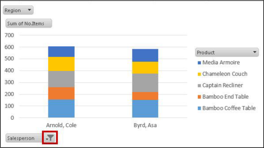
5. A filter icon will appear next to the dropdown arrow to indicate a filter has been applied to the field (See Figure 12).
  
  Figure 12 - Filter Applied
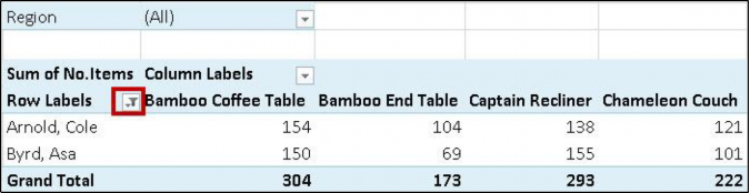
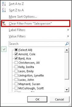
6. To remove the filter, click on the dropdown arrow.
7. The dropdown menu will appear. Click on Clear Filter From to remove the filter (See Figure 13).
Figure 13 - Clear Filter From

PivotCharts
Similar to PivotTables, PivotCharts can be used to quickly summarize, sort, filter, and analyze large amounts of data, and display that data as a visual representation. After creating your PivotTable, you can create a PivotChart using a variety of available charts (e.g. Pie, Line, Bar) that uses the same field settings.

Creating PivotCharts
The following will show you how to create a PivotChart from an existing PivotTable:
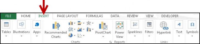
1. In the Ribbon, click on the Insert tab (See Figure 14).
  Figure 14 - Insert Tab
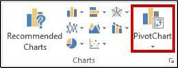
2. Under the Charts grouping, click on PivotChart (See Figure 15).
  
  Figure 15 – PivotChart
3. The Insert Chart window will appear. Select a chart from the options presented (See Figure 16).
  
  Figure 16 - Insert Chart
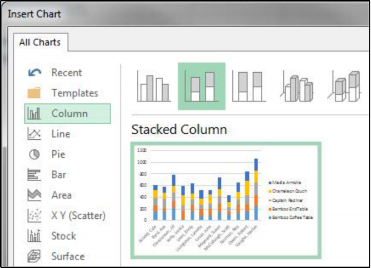
4. Click on OK.
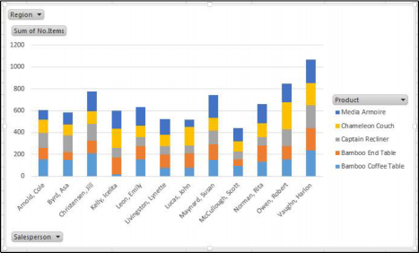
5. The PivotChart will be placed into your worksheet (See Figure 17).
  
  Figure 17 - PivotChart Inserted
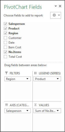
6. The PivotChart Fields will appear on the right of the screen (See Figure 18).
Figure 18 - PivotChart Fields

Note: You can alter the information that is displayed the same way as with PivotTables. See Analyzing Data with PivotTables for more information.
Filtering the PivotChart
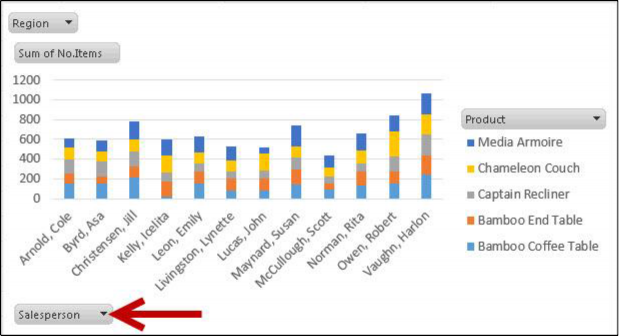
The following shows how to filter information within a PivotChart:
1. Next to a Field Header, click the dropdown arrow (See Figure 19).
  
  Figure 19 - Dropdown Button
2. A Dropdown menu will appear with values for the field listed below (See Figure 20).
  
  Figure 20 – Filter Values
3. Click the checkboxes to select/deselect values that you want to filter for.
4. Click on OK to apply your filter.
5. A filter icon will appear next to the dropdown arrow to indicate a filter has been applied to the field (See Figure 21).
  
  Figure 21 - Filter Applied
6. To remove the filter, click on the dropdown arrow.
7. The dropdown menu will appear. Click on Clear Filter From to remove the filter (See Figure 22).
  
  Figure 22 - Clear Filter From
  Using Slicers to Filter Data
  Slicers can provide greater control over your PivotTable or PivotChart when you are analyzing your data. Slicers work similar to filtering your information, but allows you to insert tables that you can use to quickly select values to filter/unfilter. They will show what is currently shown/not shown at a glance. Slicers can also be adjusted to change their size and color to make them more presentable.
  
  Inserting Slicers into your PivotTable or PivotChart
  The following explains how to insert Slicers into your PivotTable:
  1. Click within your PivotTable to select it.
  2. In the Ribbon, click on the Insert tab (See Figure 23).
    Figure 23 - Insert Tab
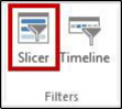
  3. Under the Filters grouping, click on Slicer (See Figure 24).
    
    Figure 24 – Slicer
  4. The Insert Slicers window will appear with a list of your available fields (See Figure 25).
    
    Figure 25 - Insert Slicers Window
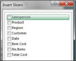
  5. Click the checkboxes next to the fields you want to create slicers for.
  6. Click on OK.
  7. The slicers will be inserted into your spreadsheet (See Figure 26).
    
    Figure 26 - Slicers Inserted
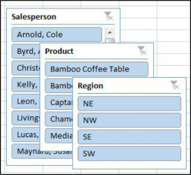
  8. Click and drag the slicers to reposition them as necessary.
  9. To apply a filter from one of the slicers, click on one of the values (See Figure 27).
    
    Figure 27 - Using a Slicer
    
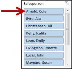
    Note: To select multiple values, hold down the shift key while clicking your values.
  10. To remove values from your slicer, click the Clear Filter icon in the upper-right corner of the slicer (See Figure 28).
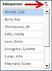
Figure 28 - Clear Filter from Slicer

Additional Slicer Options
When a Slicer is selected, the Slicer Tools – Option tab will be available in the Ribbon. From this tab, you can change the Slicer caption, style, and size of the buttons and window. To access the
Slicer Tools – Options tab:
1. Click on the Slicer.
2. In the Ribbon, click on the Slicer Tools – Options tab (See Figure 29).
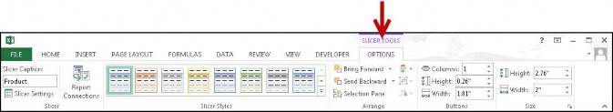
  Figure 29 - Slicer Tools - Options Tab
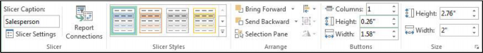
3. Additional Slicer tools will be displayed. From here you can alter the slicer captions, styles, and button and window size (See Figure 30).
Figure 30 - Additional Slicer Tools
Additional Help
For additional help mail us : support@99excel.com

Excel Service Desk for Faculty & Staff
 Phone: +91 96544-212-88
Email:
Website:

support@99excel.com

www.99excel.com